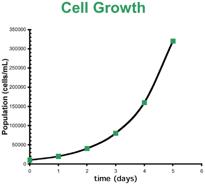
Logarithms

The Log Scale

Logarithms are not only useful in making large differences in numbers more manageable, for their use also comes in handy when one is trying to understand relationships or make predictions on graphs. Consider the following example in which an immunologist has been keeping track of the growth of some lymphocytes important for her research for 5 days:

Looking at this population explosion, the immunologist notices that the growth rate is not linear, and is in fact exponential, as she would expect. She knows the cells need to be diluted, or "split", with fresh media when they reach no more than 1,000,000 cells/mL, otherwise they will start to die from overpopulation as they exhaust the nutrients in the media. For her next experiments, she needs to make a couple of quantitative predictions.

• (1) Does she need to split her cells today (day 5) to avoid overpopulation, or can she wait until tomorrow?

• (2) She also would like to take some of her cells and dilute them into a new flask so that they are at 20,000 cells/mL after two days of healthy growth. Since the cells seemed to reach that number after one day of growth, in order to accomplish this, she needs to know how many fewer cells she should start with in her next culture so that it takes two days.

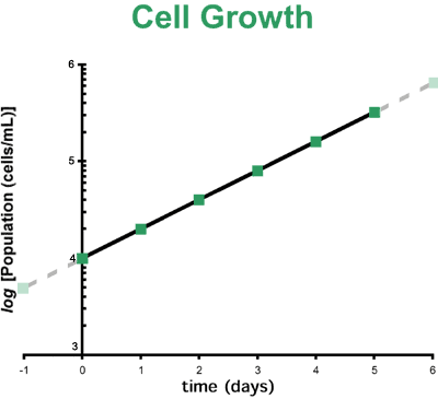
Her cell growth curve, however, is not very suited for making accurate predictions such as those needed. She needs to extrapolate both to day 6 and how many cells could have been at day "-1". Unfortunately for the immunologist, the behavior of many things in biology and chemistry are not linear, but are, in fact, exponential. Luckily, she knows that exponents and exponential trends are easily simplified by applying logarithms. So she takes her data and graphs it in a different form, using the logarithm of population as her dependent variable:

Note that the Y-axis is now in logarithmic form, so that 4 represents 10,000 cells/mL (log10,000 = 4), and 5 represents 100,000. Also note that for a log scale the marks representing intermediate values of 20,000, 30,000, etc. are not evenly spaced. With logarithmic scale you cannot say that a point measured half-way from 10,000 to 100,000 is 55,000 (it is, in fact, 31,625).

Conveniently, the immunologist's graph is now a straight line and can now be used to make her predictions. All that is needed is a straight-edge to extend the now linear trend line to tomorrow (day 6), to see if she needs to split her cells today or can wait until the morning. When she performs her extrapolation, she finds that her line extends to a little more than 600,000 cells/mL (remember, the 5 on the Y-axis represents 10,000, and the 6 represents 100,000, so the tick-marks in between are placed every 10,000 units). Therefore when she comes into work tomorrow, the population density of the cells will still be below 1,000,000 cells/mL (10⁶ cells/mL) and she can put her cell dilution off until tomorrow. Conversely, she could also extrapolate her line to find out what time she needed to split if she wanted to wait until the last moment.

Additionally, if she extends the line until day "-1", she will be able to know what starting cell density will allow her to have her 20,000 cells in two days. She determines this to be 3,333 cells/mL.

Consider the Alternative

So you see, logarithms can make math easier. Consider making these predictions reliably without the use of logarithms. The immunologist would have had to input her data and fit it to an exponential curve on a computer. Then she would have had to extract the equation of this exponential from the curve fit. The computer would have spit out this equation:

y = y₀2^x

where y₀ is the initial population at the beginning of the experiment (10,000 cells/mL) and x is the number of days of growth. Finally, she would have had to input her desired new variables for x the equation (x = 6 and x = -1) to make her predictions. As you can see, this route is much more complicated.